BigQuery Pricing: Considerations & Strategies

BigQuery (BQ) is a serverless data warehouse that allows users to query petabytes of data at high speeds. Commonly used for real-time data analytics, BQ enables stakeholders to make data-driven decisions based on proven metrics. But while BQ can help those looking to unlock the potential of data, it pays to have a sound pricing strategy, as extensive use can lead to mounting costs!

There are two main pricing components to consider:

• analysis: the cost of running queries
• storage: the cost of storing data in BigQuery

Aside from these, you should also consider Data Ingestion and Data Extraction costs. These operations are billed in two different ways: on-demand and flat-rate. The former bills operations as-is, whereas the latter is based on commitment consumption.

Executive Summary

The following concepts are essential to a complete understanding of this subject, and we will explain these further during our article. Please feel free to return here as a quick reference.

Analysis pricing	The price of running queries
Storage pricing	The price of storing data in BigQuery
Data ingestion pricing	The price of loading data into BigQuery
Data extraction pricing	The cost of extracting data from BigQuery
On-demand/pay-as-you-go billing	A pricing scheme where queries are billed as-is
Flat-rate billing	A savings vehicle where users purchase reservations at a flat price. Reservations are then used to run queries

BigQuery Pricing

BigQuery is columnar. That is, data is read and arranged using columns. The columnar nature of BigQuery shapes the way it is priced because pricing largely depends on the amount of data processed. 

A good example would be to compare a SELECT * statement with a SELECT column1, column2, and column3 statement. The former will cost the most regardless of whether or not a LIMIT clause is applied because the user selects all columns. The latter will cost less because the user is fetching only targeted columns. 

Analysis Pricing

Operations categorized as analysis pricing include queries, user-defined functions, scripts, data manipulation language (DML), and data definition language (DDL). However, the following operations are free of charge:

• load data
• copy data
• export data
• delete
• metadata operations
• read pseudo columns
• read meta tables
• creating, replacing, or invoking user-defined functions 

On-demand billing

On-demand billing is where analysis operations are billed as-is. Every month, users benefit from free queries up to 1 TB. Beyond that, on-demand queries cost $5 per TB of processed data. Data size is a summation of the data sizes of all the columns in a table.

This pricing scheme is ideal for clients who mostly run ad-hoc or non-critical workloads because BigQuery processes queries in terms of “slots.” A slot is a measure of processing capacity. Typically, up to 2,000 on-demand concurrent slots are available for each project. However, some locations might experience a high demand for slots, resulting in slower query processing time. 

The price table for data types and their sizes is as follows:

Data Type	Approximate size in bytes
INT64	8
FLOAT64	8
NUMERIC	16
BIGNUMERIC	32
BOOL	1
STRING	2
BYTES	2
DATE	8
DATETIME	8
TIME	8
TIMESTAMP	8
INTERVAL	16
STRUCT	0
GEOGRAPHY	16

Query size is calculated differently depending on the type of statement: DML, DDL, multi-statement, or clustered. The following illustrates how the query size for DML statements is applied to non-partitioned tables and how partitioned tables are calculated.

If the table is not partitioned: 

Let “q” be the sum of bytes processed for the columns referenced in tables scanned by the query. 

If the table is partitioned: 

Let “q” be the sum of bytes processed for the columns of all the referenced partitions. 

Let “t” be the sum bytes processed for all the columns in the target table.

DML statement	Bytes processed
INSERT	q
UPDATE	q+t
DELETE	q+t
MERGE	If there are only INSERT clauses: qIf there is an UPDATE or DELETE clause: q+t

For DDL statements, only CREATE TABLE… AS SELECT… statements are billed. The cost for that statement is the sum of bytes processed for all the columns referenced in tables scanned by the query.

For multi-statement queries, the following statements might incur costs: 

• DECLARE
• SET
• IF
• WHILE

These statements will only incur charges (based on the number of bytes processed) for tables referenced in the expression. 

Clustered tables will only run queries on the relevant blocks, reducing the amount of data processed. This concept is called “block pruning.” Expect lower costs for clustered tables.

Flat-rate billing

Clients with predictable workloads should use this pricing option. It works by using reservations, and the general flow for flat-rate billing is as follows:

1. The user purchases commitments
2. The user assigns slots to reservations
3. The user allocates one or more projects to a reservation

Commitments

As described above, clients will purchase something called commitments. These are slices of dedicated query processing capacity measured using BigQuery slots. A slot is a vCPU used to execute SQL queries. The number of slots needed depends on the size of the query and its complexity.

A commitment also has a duration, leading to the three types of commitment:

• Annual: lasts for a minimum of 365 days
• Monthly: lasts for a minimum of 30 days
• Flex:  lasts for a minimum of 60 seconds, typically used for testing and seasonal demands

Reservations

After the purchase of commitments, the user assigns them to different reservations. This method of resource allocation allows users to associate commitments with other workloads. Once complete, one or more projects, folders, or organizations must be assigned to a reservation to make the slots usable.

Cost table

Type of commitment	Number of slots	Pricing
Monthly	100	$2000
Annual	100	$1700
Flex	100	$4 per hour or $2920 per month

Storage pricing

As the name suggests, storage pricing is simply the cost of data storage, which is billed via two categories:

• Active storage
• Long-term storage

Active storage refers to tables or table partitions modified over the last 90 days. Long-term storage refers to tables or table partitions that have not been modified during the previous 90 days and are 50% cheaper than active storage. The first 10GB of data storage is always free.

The price table for storage is as follows:

Storage type	Pricing per month
Active	$0.02 per GB
Long-term	$0.01 per GB

Pricing is prorated at the MB level. For example, assuming that the storage is long-term, 100 MB is worth a tenth of $0.01 or $0.001. The same concept applies to Active storage.

The following actions count as modifications and therefore result in active storage:

• loading data into a table
• copying data into a table
• writing query results to a table
• using data manipulation language (DML)
• using data definition language (DDL)
• streaming data into the table

Data ingestion pricing

The data ingestion price depends on operation and data size. Batch loads from GCS or local machines are free for shared slot pools, and data ingestion is also free while a slot pool is available. If a customer purchases commitments, they then have a guaranteed slot for ingestion. 

The price table for data ingestion operations can be found below.

Operation	Price
Batch loading	Free
Streaming inserts	$0.01/200 MB
BigQuery Storage Write API	$0.025/1 GB

Data extraction pricing

There are two modes of data extraction: batch export and streaming reads. Batch export is when data is exported to Cloud Storage as a file. A streaming read is when the Storage Read API is used to read data via streaming.

Batch export: Like batch loads, batch exports are free by default because they depend on shared slots. However, slot availability is not guaranteed unless dedicated slots are purchased, and flat-rate pricing will then be applied. If a query request is made where insufficient slots are available, BigQuery simply queues individual work units until more become available.

BigQuery Storage Read API: Pricing differs depending on the regions that data is read from and to. You should also consider whether the data is being moved within Google Cloud or not, as internal movement is cheaper. For same-location egress, there is a 300 TB per month free usage limit for streaming reads. Beyond that, a $1.1 per TB data read rate is applied.

The price table for API usage within Google Cloud is as follows:

Case	Pricing per GB
Accessing query results from temporary tables	free
Data reads within a location	free
Data reads from multi-region to a site in the same continent	free
Data read from different locations within the same continent	$0.01
Data read between different continents (except Australia)	$0.08
Data read between Australia and a different continent	$0.15

The price table for API general network usage is as follows:

Monthly usage in TB	Egress to worldwide destinations (except Asia and Australia)	Egress to Asian destinations except China, but including Hongkong	Egress to Chinese destinations (except Hong Kong)	Egress to Australia	Ingress
0-1	$0.12	$0.12	$0.19	$0.19	free
1-10	$0.11	$0.11	$0.19	$0.18	free
10+	$0.08	$0.08	$0.15	$0.15	free

Recommendations

To reduce your bottom line, we endorse the use of several cost-saving strategies, which are listed below.

Use partitioned and clustered tables where possible

Due to “block pruning,” the amount of data processed per query for these tables is less on average compared to unpartitioned and unclustered tables. Block pruning is when only relevant blocks in a table are scanned. You can achieve this by limiting queries using the WHERE clause.

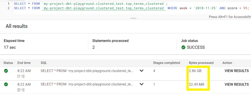
To illustrate this concept, we can create a clustered table like so:

Then, we run two queries. The first query does not use a WHERE clause, but the second uses WHERE to filter by week and score. Based on the performance summary below, our first query scanned 2.86 GB of data, whereas the second only ran through 22.49 MB.

Take advantage of cost controls

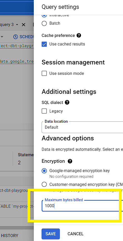
Use a setting called maximum bytes billed to limit the amount of data processed. If a query goes beyond this value, the query will fail without incurring costs. To do this, simply go to Query settings and Advanced options before running your statement.

Regularly examine audit logs

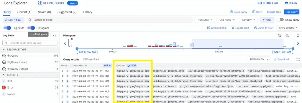
Queries are logged automatically by Cloud Audit Logs, which contain pertinent information such as the query statement, duration, and cost. You can also stream audit log data in real-time, enabling you to gather live cost metrics. Usage patterns are also described, providing insights that can be vital when developing a cost optimization strategy. These include CPU and memory consumption metrics that you can use to identify a baseline of required resources.

Estimate storage and query costs

Before running queries, you should obtain an estimate of possible costs by using the following resources:

• query validator within the console
• bq command-line tool with the –dry_run flag
• API with the dryRun parameter enabled
• Google Cloud pricing calculator
• client libraries

Before running queries on the console, a small text field indicates how much data will be processed, and this is the easiest way to estimate query costs. Please see the image below for reference.

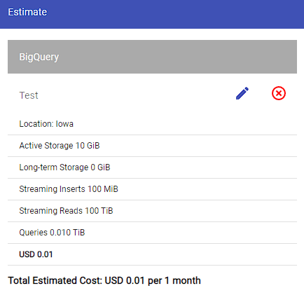
The two methods discussed above are usually sufficient for most cost estimation needs. Other options exist but are typically used for particular situations. For example, the bq command-line tool is generally used by developers who use Cloudshell as an IDE. The API and client libraries are primarily used within Python, Go, Java, Node.js, and PHP scripts. 

Conclusion

BigQuery pricing has two pricing components: analysis and storage. As we have seen, analysis costs are necessary to run queries, and storage costs are incurred when storing data on BigQuery. Furthermore, there are separate costs for data ingestion and extraction operations. 

The two BQ pricing models are on-demand and flat-rate. On-demand pricing generates costs as queries are run (defined by the relevant pricing table). On the other hand, flat-rate billing can be described as a savings vehicle where a user purchases consumable slot commitments. 

We recommend these best practices to help optimize and reduce your query costs: use partitioned or clustered tables, take advantage of cost controls, regularly examine audit logs, and estimate storage and analysis costs before running live queries.

We hope you have enjoyed reading this article and found it helpful in further developing your BQ pricing strategy!